In my previous article, The Neural Network Cost Function, I describe the cost function and highlight the essential role it plays in machine learning. With the cost function, the machine pays a price for every mistake it makes. This provides the machine with a sort of incentive or motivation to learn; the machine's goal is to minimize the cost by becoming increasingly accurate.

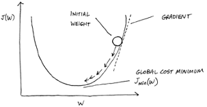
Unfortunately, the cost function tells the network only how wrong it is; it doesn't provide a way for the network to become less wrong. This is where machine learning gradient descent comes into play. Gradient descent is an optimization algorithm that minimizes the cost by repeatedly and gradually moving the output in the direction opposite of that in which the slope of the gradient line increases, as shown here. 

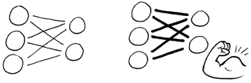
During the learning process, the neural network adjusts the weights of the connections between neurons, giving input from some neurons more or less emphasis than inputs from other neurons, as shown below. This is how the machine learns. With gradient descent, the neural network adjusts the initial weights a tiny bit at a time in the direction opposite of the steepest incline. The neural network performs this adjustment iteratively, continually pushing the weight down the slope toward the point at which it can no longer be moved downhill. This point is called the local minimum and is the point at which the machine pays the lowest cost for errors because it has achieved optimum accuracy.

For example, suppose you are building a machine that can look at a picture of a dog and tell what breed it is. You would place a cost function at the output layer that would signal all the nodes in the hidden layer telling them how wrong the output was. The nodes in the hidden layer would then use gradient descent to move their outputs in the direction opposite of the steepest incline in an attempt to minimize the cost.

As the nodes make adjustments, they monitor the cost function to see whether the cost has increased or decreased and by how much, so they can determine whether the adjustments were beneficial or not. During this process, the neural network is learning from its mistakes. As the machine becomes more accurate and more confident in its output, the overall cost is diminished.

For example, suppose the neural network's output layer has 5 neurons representing five dog breeds — German shepherd, Doberman, poodle, beagle, and dachshund. The output neuron for the Doberman indicates a 40% probability the picture is of a Doberman; the German shepherd neuron is 35% sure it's a German shepherd; the poodle neuron is 25% sure it's a poodle; and the beagle and dachshund neurons each indicate a certainty of 15% the picture is of one of their breeds.

You already decided that you want the machine to be 90% certain in its analysis, so these numbers are not very good.

To improve the machine's accuracy, you can combine the cost function with gradient descent. With the cost function, the machine calculates the difference between each wrong answer and each correct answer and then averages them. So let’s say it was a picture of a Doberman. That means you want to nudge the network in a few places:

• +0.60 for the Doberman to get it to 1.0
• -0.35 for the German shepherd to get it to 0.0
• -0.25 for the poodle to get it to 0.0
• -0.15 for the beagle and dachshund to get those to 0.0

Then you want to average of all your nudges to get an overall sense of how accurate your network is at finding different dog breeds:

(+0.60 – 0.35 – 0.25 – 0.15 – 0.15)/5 = –0.55/5 = –0.11 

But remember this is just one training example. The machine repeats this process on numerous pictures of dogs of different breeds:

(0.01 – 0.6 – 0.32 + 0.16 – 0.25)/5 = –0.04/5 = –0.02

(0.7 – 0.3 + 0.12 – 0.05 – 0.12)/5 = 0.35/5 = 0.07

With each iteration, the neural network calculates the cost and adjusts the weights moving the network closer and closer to zero cost — the point at which point the network has achieved optimum accuracy and you are confident in its output.

As you can see, the cost function and gradient descent make a powerful combination in machine learning, not only telling the machine when it has made a mistake and how far off it was, but also providing guidance on which direction to tune the network to increase the accuracy of its output.