An artificial neural network requires several components to drive its machine learning process, including the following:

• Artificial neurons: Commonly referred to as "nodes," artificial neurons are like brain cells. Each neuron receives one or more inputs and performs a calculation on those inputs to produce an output.
• Weights: Weights are added to the connections between neurons to control the relative importance of each neuron's output. For example, suppose you have an artificial neural network designed to tell whether a person is smiling or frowning. You would want to place more weight on inputs related to the person's mouth and eyes and less weight on inputs related to their nose, chin, and hair.
• Biases: Bias is similar to weight, but it is an adjustment made within a neuron to control its output.
• Activation functions: The activation function, within each neuron, is responsible for performing a calculation on the sum of the weighted inputs to produce the neuron's output.
• Cost function: The cost function resides at the end of the neural network and calculates the difference between the network's answer and the correct answer. In other words, it determines how wrong the artificial neural network is.
• Gradient descent: Gradient descent is a technique that tells the artificial neural network the adjustments required to bring the answer closer to the correct answer. See my previous article Fine Tuning Machine Learning with Gradient Descent for details.
• Backpropagation: Neural Network Backpropagation calculates the gradient of the cost function at output and distributes it back through the layers of the artificial neural network, providing guidance on how to adjust the weights to increase the accuracy of the output. Think of weights and biases as dials that can be turned to adjust each neuron's output. Backpropagation provides guidance on which dials to turn, in what direction, and by how much.

Turning Dials

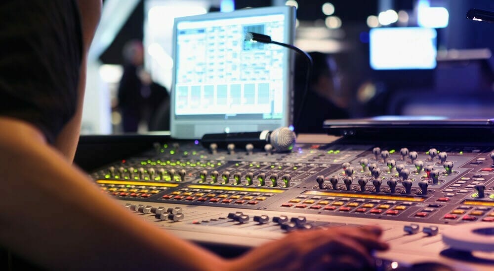
To understand how backpropagation works, imagine standing in front of a control board that has a few hundred little dials like the ones you see in professional sound studios. You’re looking at a screen above these dials that has a number between one and zero. Your goal is to get that number as close to zero as possible — zero cost. You don't know anything about the purpose of each dial or how its setting might impact the value on the screen. All you do is turn dials while watching the screen.

When you look closely at these dials, you notice that each has a setting from 0 (zero) to 1 (one). Turning a dial clockwise brings the setting closer to one. Turning it counter clockwise brings the setting closer to zero. Each dial represents a weight — the strength of the connection between two neurons. It’s almost as though you’re tuning an instrument without actually knowing the notes. As you make adjustments, you get closer and closer to perfect pitch, at which point the cost is zero.

With an artificial neural network, the dials start with random settings, which allow them to be turned up or down. During the training process, the network looks for the dials with the greatest weights — the dials that are turned up higher than all the others. It turns all of these dials up a tiny bit to see if that lessens the cost. If that adjustment doesn’t work, the network turns them down a little.

Example

Suppose we build an artificial neural network for identifying dog breeds. It is designed to distinguish among 10 breeds: German shepherd, Labrador retriever, Rottweiler, beagle, bulldog, golden retriever, Great Dane, poodle, Doberman, and dachshund. We feed a black-and-white image of a beagle into the machine.

This grayscale image is broken down into 625 pixels in the input layer, and that data is sent over 12,500 weighted connections to the 20 neurons in the first hidden layer (20 x 625 = 12,500). The first hidden layer neurons perform their calculations and send the results over 400 weighted connections to 20 neurons in the second hidden layer (20 x 20 = 400). Those second hidden layer neurons send their output over 200 weighted connections to the 10 neurons in the output layer (20 x 10 = 200). So our network has 13,100 dials to turn (12,500 + 400 + 200 = 13,100). On top of that it also has 50 settings to adjust the bias in the hidden and output layer neurons. All the weights start with random settings.

We send our beagle picture through the neural network, and the output layer delivers its results; it’s 0.3 certain it’s a German shepherd, 0.8 sure it’s a Labrador retriever, 0.5 sure it’s a Rottweiler, 0.2 sure it’s a beagle, 0.3 sure it’s a bulldog, 0.6 it’s a golden retriever, 0.3 sure it’s a Great Dane, 0.3 sure it’s a poodle, 0.4 sure it’s a Doberman, and 0.7 sure it’s a dachshund.

Obviously, those are lousy answers. The network is much more certain that the picture of the beagle represents a Labrador retriever, a Rottweiler, a golden retriever, or a dachshund than a beagle.

The neural network needs to use backpropagation to find out how to adjust its weights and minimize the cost. The best place to start is by dialing up the correct answer (beagle), because it’s the right answer and it has the most room for adjustment; that is, you can dial it up more than you can dial the others up or down. The next priority is to dial down the wrong answers starting with the highest number, so you would start by dialing down the 0.8 (Labrador retriever) and the 0.7 (dachshund).

So backpropagation looks at 0.2 and works its way back to the connections to this output neuron to identify which connections have the most room for adjustment, and it dials those up or down. It then looks back to the second hidden layer neurons to see which neurons have the most room to adjust the bias, and it dials those up or down. The network continues to work back through the connections and neurons and continues to make adjustments until it reaches the input layer.

As you can see, backpropagation is a powerful technique that enables machines to learn as we often do as humans — through trial and error. We make mistakes, analyze the outcome, and then make adjustments to improve the outcomes. If we don't, we pay the high cost incurred from continually making the same mistakes!